How Markets Work

Modern financial markets run on a continuous double auction system to match buyers and sellers.  Market orders to buy and sell can be matched when they arrive simultaneously or within a very narrow time window.  These buyers and sellers have their orders executed at a "market price" that theoretically should be within the spread of the best bid and asked prices in the limit order books.  It is a double auction because simultaneously limit orders to buy and sell are arriving and being sorted by price and arrival time into the limit order books.  Limit orders can also be removed by the participant who placed the order and limit orders are removed as the market price moves above or below those prices in the limit order books such that the limit orders become market orders.  The graphic below shows a simplified cartoon of the process at a single instant with a market price of 50.  Imagine a series of these cartoons as a movie with the orders flowing in, limit order book frequency plots changing and the price dynamically moving on the abscissa, while the market is churning out at the bottom a price time series.

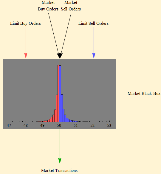
It is essentially a black box, because we never know in real time the flow rates of the orders, and we never know the full structure of the limit order books, but we know some of the algorithmic rules and studies have shown that the structure of the limit order books have implied heavy tailed returns, well fit by a power tail.  In the simplified model, orders flow into the system in two types, market orders which are executed as soon as possible over a very short time interval and limit orders which are sorted by price and time into order books and filled on a first come first served basis when the price limit is reached in the market.  When numbers of buy and sell market orders are equally matched, the orders are executed at the current market price and each party is charged a commission on top of the market price.  The market price does not change and the return over this interval is zero.  If the market orders are not equally matched, then the unmatched buy or sell orders are filled in the respective sell or buy order books and the price changes, generating positive or negative returns.  In reality there are a number of these markets running simultaneously and there are more complicated order instructions that can be placed in each of these markets.  The structure of the order flow rates is dynamic and not known, and the structure of the limit order books is not likely static.

There is a lag in transmission of the executed price information, across networks, and prices may be executed in different markets and on different servers.  So for some brief interval which now may be measured in hundreds of milliseconds to several seconds, one trader is not aware of the actions of other traders.  There is also a lag in the execution of orders, so it is likely that over very short time frames of several seconds, market prices and the implied returns are independent and random.  But over periods of time longer than a few seconds trading behavior is not independent.  As price change information is disseminated, flow rates of orders and order cancellations change and the structure of the order books.

If in some very brief time interval the order structure is static and orders arrive in independent fashion,  then the sums of independent identically distributed logarithmic returns would converge to a stable distribution, by the generalized central limit theorem.  For this to succeed there must be a sufficient number of transactions.  Market orders generate an excess of zero returns, but these disappear on summation with other returns.  If the order books have a static heavy tailed return distribution, the result of the summed logarithmic returns, will be a stable distribution with alpha less than 2.  Otherwise the summed returns seen in the market transactions would be normally distributed.

Studies have shown that the structure of the limit order books have heavy power tails, but we do not know how stationary this structure might be.  If the structure is not stationary over time then the resulting distribution of returns flowing out of the market will not be identically distributed.  If the flow rates of market orders increase faster than the flow rate of limit orders then mismatched market orders will penetrate deeper into the order books and the scale factor of the distribution of returns will change dynamically; this activity will also cause returns not to be identically distributed.

As information about transacted prices is disseminated, traders act on this information and a structure of dependence develops in the returns, so they are no longer independent.  As the returns lose their independence and their distributions are no longer identically distributed, they will no longer be described by the generalized central limit theorem.

Market Transactions

We do not easily have access to the structure of the market order books and flow rates, but we can usually find information about every transacted price.  Typically since these occur with high frequency, we are given the results over a brief interval like a minute with the opening price for the interval, the high and low price for the interval, and the closing price of the interval.  We also usually have the volume of transactions of shares over the interval.  We can easily obtain this data within seconds of its occurrence in the form of "real-time" quotes.

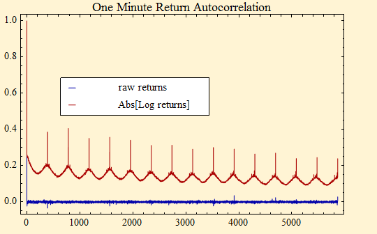
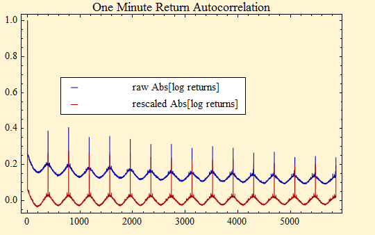
The plot below shows a plot of autocorrelation function of one minute returns for the SPY ETF collected from July 2007 through March 2009, for a lag of 15 days of one minute returns.  The numbers on the x-axis are trading minutes.  The blue plot is the autocorrelation function of the raw logarithmic return data.  It shows no evidence of serial dependence, but when the autocorrelation plot is done with the absolute value of the returns, a rich dependent structure immediately appears, shown in red.  The data are concatenated so that each day begins with a larger than one-minute return that occurs from the previous market close to the market open. This is the cause of the repeated spikes in the red autocorrelation plot.   There also can be seen in the red curve a cyclic structure that occurs through out the day in a rather regular pattern.  The absolute value of the returns is the simplest measure of volatility; thus we see that volatility is changing dynamically with a serially dependent structure each minute of the day.  The largest spike in the cyclic structure occurs at the market open, volatility is higher in the early hours, it falls to a low at mid-day, then rises until the market close.  This cycle recurs every day.  There is also a dependent structure from one day to the next that decays very slowly.

The cyclic nature of the volatility structure gives us the idea of looking at each day's data and analyzing it with stable distributions despite the fact that we know the returns are not independent.  The idea is that since each day repeats the same cycle, perhaps fits from one day to the next will behave like an average stable distribution for each day.  When we do the stable parameter fits to each day's minute return data and average them we get the stable parameter results shown below.

α	β	γ	δ

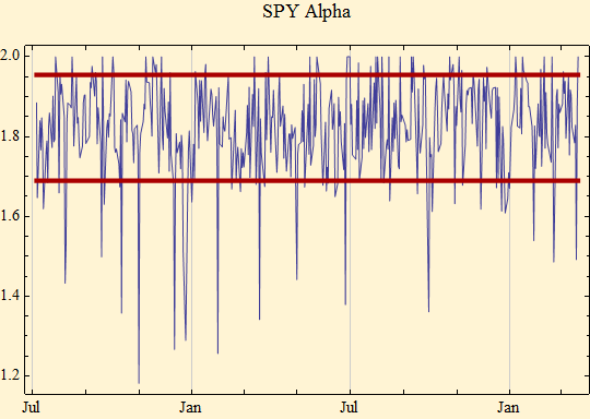
Next is a plot in blue of the alpha parameter for each day's data.  Alpha is the stable distribution shape parameter and it is also the tail exponent of the distribution.  The red lines are the 95% confidence bands for the technique around the mean alpha shown above.  Not all the trading days are equal in length due to holidays; this and the knowledge that the data within each day are not fully random, may explain some of the wide excursions outside the 95% confidence intervals.  The data nevertheless suggest that there is a somewhat stationary tail exponent to the distribution of market returns from day to day.  Could this be the same tail exponent in the market limit order books?

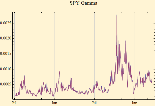
When we look at the day to day variation of the gamma parameter we see a very different picture.  The graph contains two curves one red and one blue.  The blue method of determining gamma uses a maximum likelihood method to calculate all the stable parameters and the red uses a very fast characteristic function method to fit only the gamma parameter to each day's data.  The results shown in the graph are nearly identical.  The gamma parameter is the scale factor of the distribution.  Note that the range of variation is ten fold over the period studied.  Stable distributions retain their shape on scaling so each day's data could be standardized by dividing the day's returns by the scale factor of the day.

We do this division and re-examine the autocorrelation function.  The rescaled data is now in red.  We see that the intraday cycle remains and the inter-day spike is retained, but the serial dependence from one day to the next disappears.  The average autocorrelation over the daily cycle is approximately zero.

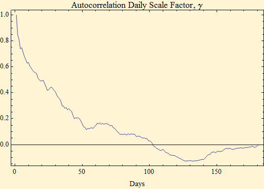
We guess that we may have captured the inter-day serial dependence in the gamma parameter to the stable fit.  So we look at the autocorrelation function of the day to day gamma parameters.  The lags shown on the x-axis are now trading days instead of trading minutes.  We now have a very strong pattern of serial dependence with a lag of over 100 days.

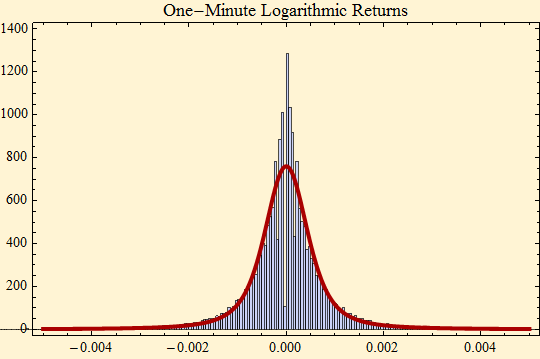
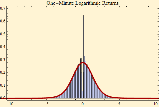
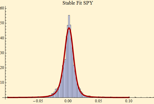
We could also try to remove the intraday cycle, but a look at the entire data set as raw data and rescaled data suggests that this may not be necessary.  Below are the parameters fitting the raw return data to a stable distribution.  The histogram is shown along with the fit and a log-log plot of the empirical distribution function and fit are shown to examine the tail behavior.  First we note that alpha is considerably lower than the average alpha obtained from fitting each day separately.

α	β	γ	δ

Next we notice that the density histogram has too much mass in the middle for the calculated stable density.

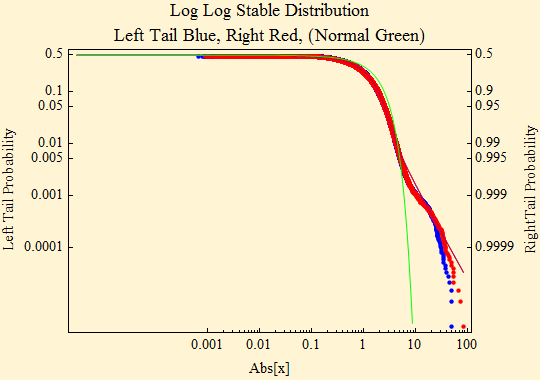
Below is a log-log plot which fits the data to the stable distribution function with parameters from the maximum likelihood fit. There are five plots in this illustration, three of which are lines representing the tails of distributions implied by parameters and two of which are plots of actual data.  To align the tails, the absolute value of the left tail is shown in blue; the right tail is shown as 1 - probability in red.  Displayed this way a stable distribution with α < 2, reflects linear parallel tails with the slope of minus α.  If β is zero the tails are superimposed.  The tail of a Normal distribution, defined by its first two moments calculated from the sample, is shown in green and is not linear.  The dots show the data points of the two respective tails.  In this representation, stable distributions have a characteristic shape with parallel tails that become linear when α≠2; except when β = ±1, in which case the lighter tail is not linear.

The divergence of the data points from the theoretical tails in the log - log plot illustrates the fact that the maximum likelihood stable fit to the data does not handle the tails very well.  The tail exponent, α, shows up with a slope of minus α in this plot.  The slope of the fit, -1.38, is considerably lower, less steep, than the slope of the data.

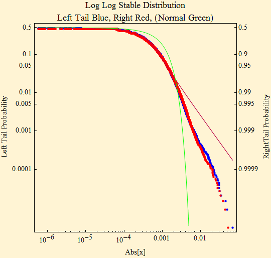
This finding on the tails is typical of stable fits to market data at other time scales such as daily data.

Next we show the fits to the whole data set when each day's data is divided by the gamma parameter calculated for that day.  Alpha is now close to 1.8 and is thus consistent with the average alpha found when each day's data are fit individually.  Since we have rescaled each day to a gamma of 1.0, gamma found for the whole data set is close to one as should be expected.  

α	β	γ	δ

The histogram now shows a much better fit to the rescaled data.  The large spike is caused by an excess of zero returns in the one minute data set: these remain zero upon division by the scale factor and show up as a single prominent spike in the histogram.

The tail fit to the rescaled data is nearly perfect.

Our hypothesis is that on some very short time scale market behavior is independent and identically distributed.  This time scale may be on the order of a fraction of a second for a program trading algorithm, but would be considerably longer for a human trading with a delay for transmission and assimilation of data and additional delay for reaction time and execution time for the order.  We guess that there is a spectrum of independence for different market participants, but out analysis of the data suggests that at the one-minute sampling interval, we may be seeing data that is obeying the generalized central limit theorem and converging to a stable distribution.  This stable distribution, however, does not have stationary parameters and we can see that the structure changes on a minute by minute basis through the day by the autocorrelation function, yet when we fit each day's worth of minute returns, it seems that we can come up with an average scale factor, gamma, for the day.  When we correct the large data set for this variation in scale factor we get a very good fit to a stable distribution.

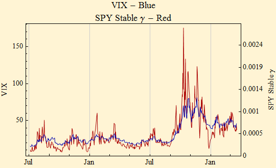
Going back to the black box of the continuous double auction model, we suspect that the tail exponent in the limit order books must be relatively static for us to see such an alpha-stable phenomenon.  Our idea is that market returns can be well modelled by alpha stable noise multiplied by a scale factor that varies from minute to minute during the day and has a strong serially dependent structure.  This is the varying scale factor of a non-stationary stable distribution.  This parameter is not independent or random.  It is the volatility signal given off by the market.  To illustrate that idea further we show a daily plot of the CBOE VIX along with stable gamma.

The Structure of Volatility

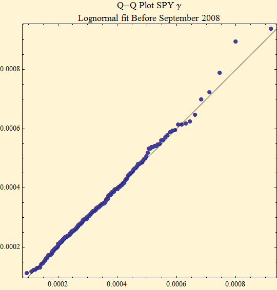
When we look at the volatility tracings in the above graphic, we can imagine repeated cycles of rises in volatility followed by slower decays.  Before September 2007 in our study the cycle pattern appears regular.  After the extreme rise in volatility seen in September 2007,  reaching a peak in October there seems to be a very slow decay in volatility with perhaps a cyclic structure superimposed on that decay.  As we studied the phenomena before September 2007 we noted that the histogram of the daily volatility parameters was well fit by a lognormal distribution.  Below is the histogram and parameters for a maximum likelihood lognormal fit.  The quantile - quantile plot also suggests that the data are well fit by a lognormal model.

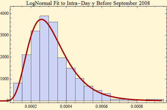
MLE fit to lognormal distribution, log likelihood and parameters

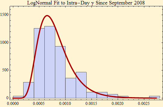
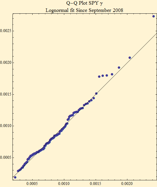
As we added data after September 2007, we noted that the lognormal model broke down.  But now that we have more data, we find that the lognormal fit to the data after September 1, 2007, also is reasonably well fit by a lognormal distribution.  The parameters of the fit have changed.

MLE fit to lognormal distribution, log likelihood and parameters

These are interesting findings, but they may not be mathematically useful, because the distributions seen in the histograms are not random.  The meaning behind the lognormal finding may simply be the decay periods seen in the cycles of volatility are logarithmic in nature and the errors to the fit of the logarithmic function are simply normally distributed.  If we presume that the cycles over many hundreds of days or years have a relatively random, then we might be able to fit returns on the scale of days to a stable mixture distribution, where the gamma parameter is lognormally distributed.  

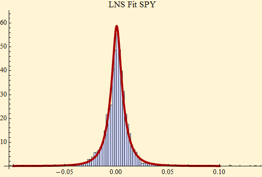
Our initial attempts at this appear somewhat promising.  The lognormal stable (LNS) mixture distribution adds a fifth parameter, σ, which corresponds to the standard deviation of the log of the scale factors.  However, when we are dealing with daily interval data, we do not know the intraday information, so we try to reconstruct them by looking at a the data partitioned into subsets of 30 trading days and estimate these parameters from the partitioned data, hoping that the slow decay of volatility won't matter too much.  When we rescale each partition with the estimated gamma for the partition, we get a better fit to the tail exponent of the daily data than we do with a raw stable fit.  The fit below takes daily trading data from Fri 29 Jan 1993 through Fri 20 Mar 2009.

The result is a higher α, than we would get using a stationary stable fit, and encouragingly this is very close to the result we get for the intraday data.  The parameters we use in the final fit are α and β from the rescaled stable calculation, γ and σ are taken from the above fit to the scale factors at 30 day intervals, and δ is the mean of all the returns.  A Fast Fourier Transform method is used to calculate the LNS density and we reuse this later to quickly calculate the log likelihood of the fit parameters, {α, β, γ, σ, δ}.

{1.82391, -0.0606083, 0.00572723, 0.592975, 0.000206468}

{1.55853, -0.172732, 0.00608439, -0.0000639102}

Comparing the two fits, we see that the LNS fit handles the peak of the distribution better and the tail exponent α is higher so that the parameters would be less likely to over-estimate extreme events if they are used for simulation.  Below, the log likelihood is calculated for the stable fit and the LNS fit which is higher.

Stable log likelihood: 12594.3

LogNormalStable log likelihood: 12608.8

© Copyright 2009 Robert H. Rimmer  Sat 21 Mar 2009