Stable PRNG
The stable pseudorandom number generator provides some insight into the behavior and structure of stable random variables and contains the necessary formulas to compute stable probabilities. This page will demonstrate the algorithm when α ≠ 1, for the standardized 1-parameterization. The basic algorithm in Mathematica is shown below.

u1 and u2 are independent uniform random variables with a range (0, 1). As such this function can also be thought of as a two dimensional inverse quantile function for stable distributions spread over a unit square. It also shows that stable random variables can arise as the product of two random variables. This idea will be explored in more detail below.
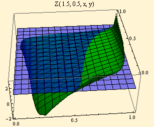
The 3D plot below shows the function Z for α = 1.5, β = 0.5 in green. A plane set at Z = 1 is shown in blue. The x and y axes of the graph range from zero to one, thus the blue plane has an area of one. The plane cuts the green plot in such a manner that the area of the square to the left of the cut is the probability of Z ≤ 1. The contour of the cut is the Zolotarev integrand for the stable distribution function scaled to have its domain constrained by the unit square.
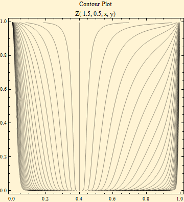
The curves from the integrand are shown as contours on the unit square in the graph below. The stable probability function could be calculated as the area to the left of the curve using an indicator function, ![]() , which returns 1 if Z ≤ z and 0 otherwise.
, which returns 1 if Z ≤ z and 0 otherwise.
![]()
But usually it is easier and more accurate to calculate the area under the curve and subtract from 1.
Note also that there is one vertical curve in the group, this is at Z = 0, where there is a known function for the distribution function, for α ≠ 1.
![]()
The lower portions of the curves converge to this vertical point, when α > 1.

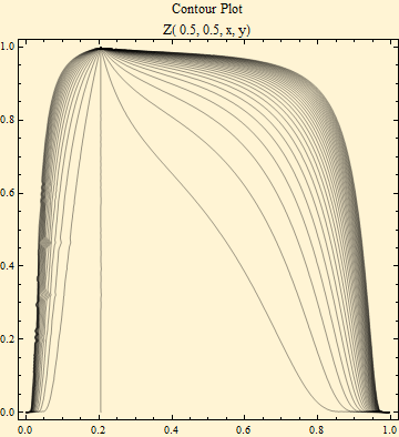
When α < 1, the convergence to the line is in the other direction.

The formula can be rewritten so that Z is the product of two random variables, each based on an independent uniform random variable, q and p. The separate formulas are quantile functions for each random variable.

The formula for the q component can be solved to a distribution function.

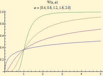
This distribution function is a variant of the Weibull and Fréchet extreme value distributions. A plot is shown below for curves where α = {0.4, 0.8, 1.2, 1.6, 2} from bottom to top.
The distribution function for the other component, p, cannot be solved, but it can be plotted as an inverse quantile function.

Plots for this distribution function are shown below for the symmetric case and the same α’s. This component of the random variable determines the sign of Z and most of the tail behavior. For the normal stable case when α = 2 the distribution is finite and has a formula.
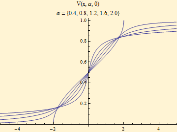
For the normal stable case when α = 2, the distribution is finite and has a formula.
![]()
In that case the tail behavior is determined by W (x, 2).
![]()
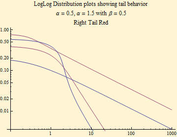
The loglog plot below shows the Pareto tail behavior of the function, V, when α < 2. Calculations of this show that the negative slope of the loglog plot matches α.
We have shown the operation of the stable pseudo random generator and that stable random variables are generated as a product of two random variables, one belonging to a light tailed extreme value type of distribution with a tail exponent of ![]() and the other of a peculiar distribution derived from the Zolotarev transform of the Fourier transform of the stable characteristic function. This latter distribution determines the sign and tail exponent of the stable random variable.
and the other of a peculiar distribution derived from the Zolotarev transform of the Fourier transform of the stable characteristic function. This latter distribution determines the sign and tail exponent of the stable random variable.

© Copyright 2011 mathestate Fri 17 Jun 2011
