A New View of Risk

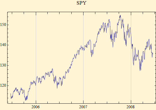
The lognormal - normal mixture distribution (LNN) gives a very good fit to financial data.  Its parameters also provide an new insight into risk.  We have defined three parameters for the distribution, {γ, σ, δ}.  γ and δ are analogous to the stable scale factor and location parameter, with δ also being the expectation of the distribution.  Since our distribution is of logarithmic returns, δ is the expected logarithmic return.  We will start with some data.  Three years of SPY.

LNN Parameters {γ, σ, δ} = {0.00485112, 0.541252, 0.000604314}

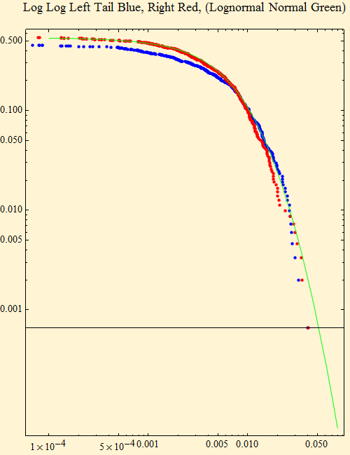
Here is the log-log fit.  The data has some asymmetry, but this is a symmetric distribution, nevertheless the risk at the tails in the data is well described by the distribution.  Click this link for gallery of fits to data of all the stocks in the Dow Jones Industrial Average.

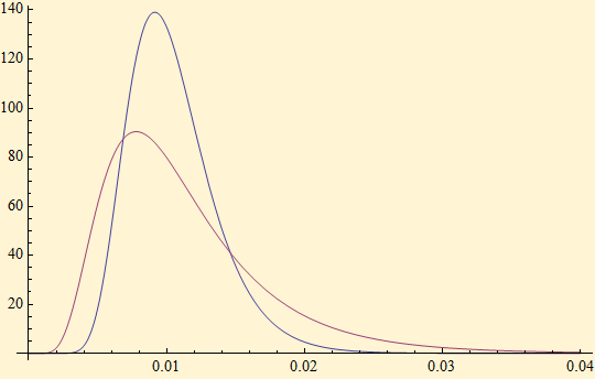
Below are the plots of the two densities that create our distribution function.  The concept of LNN is that it describes a random variable a product of a random variable from each of these two distributions.  The normal distribution on the left has its mode at the mean, 0, and its scale factor is adjusted to the stable scale factor of 1.  The lognormal distribution is characterized by parameters μ, and σ.  In the LNN representation μ is given the value log(γ) and σ is the same as our σ parameter.  Thus the risk is uniquely pictured in the density of the lognormal distribution, which tells something about the shape of volatility.

The normal distribution random variable has constant parameters.  It adds a noise factor to the lognormal random variable which has two parameters that characterize the risk.  This noise is a product not an addition so its effect to significantly broaden the mass of the tails of the distribution.  All of the risk in the LNN distribution is represented by the lognormal distribution parameters.  The x-axis of the lognormal distribution represents the scaling of the normal distribution noise and the y-axis is the weight assigned to the value on the x-axis.  The following relationships describe the lognormal part of the distribution.

γ is the median of the lognormal distribution.

The mode is located at γ .

The expectation of the lognormal distribution is .

The standard deviation of the lognormal distribution is γ .

Thus if σ were 0 the scale factor of the stable noise would be γ and there would be no dispersion of the noise.  As σ grows the risk is spread out.  The graph below shows the lognormal distribution with γ set to 0.01 and σ at 0.3, blue, 0.5, red.

As σ grows the risk multiplier has more extreme events in its probability distribution.  On the next page we take up generation LNN Random variables.

© Copyright 2008 mathestate    Wed 18 Jun 2008