StableConvolution

Stable Convolution

The convolution of two statistical densities gives the density of the sum of random variables from the two distributions. A convolution of a density with itself gives the density of the sum of two random variables from the distribution. The convolution of a stable distribution with itself, gives a stable distribution with the same shape and skewness, {α, β}. In the 1-parameterization the changes to γ and δ are straight forward. Where n is the number of convolutions, the scale and shift changes with convolution are:

But convolution is also a smoothing operation, suggesting that there may be a place for this in data analysis. Consider the empirical characteristic function:

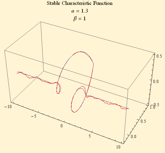
Below is the plot of a stable characteristic function in three dimensions in blue. In red is the plot of the empirical characteristic function of a stable random sample with the same parameters. The sample size is 1000.

Graphics:Stable Characteristic Function α = 1.3 β = 1

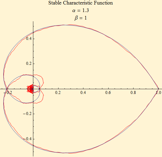
Each random variable can be imagined as an orbit in the complex plane. The orbit of the characteristic function of a single random variable is the unit circle with the value of the random variable determining the speed and direction of the orbit. When you take the mean of these orbits, you have the orbit of the characteristic function. Viewing the above plot only in the complex plane, you see the orbit at t = 0 at position 1 + 0 i, as t goes to ±∞ the orbit spirals to the origin. Looking at the picture it is clear that the tail of the empirical characteristic function is not so smooth at the portion near t = 0.

Graphics:Stable Characteristic Function α = 1.3 β = 1

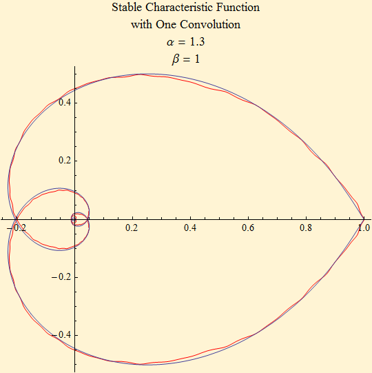
The graph below shows the empirical characteristic function convolved with itself. There is smoothing of the tail, but some distortion of the mid portion of the function.

Graphics:Stable Characteristic Function with One Convolution α = 1.3 β = 1

The CFFit routine in StableM currently uses a convolution of the empirical characteristic function with a negative version of the sample to symmetrize the distribution for fitting α and γ, but it does not yet take advantage of the smoothing to use more of the tail of the characteristic function. Below is a version CFFit1 that doubles the tail length. Most of the time the fit is marginally better with this enhancement, but not usually so good as the much slower maximum likelihood fit. The log likelihoods are shown for each of the fits.

p1 = CFFit[s]
p2 = CFFit1[s]

SLogLikelihood[s, p1]
SLogLikelihood[s, p2]

p3 = SFit[s]
SLogLikelihood[s, p3]