Empirical Characteristic Function

An empirical characteristic function can be defined as below, where {, , ... } is a sample of i.i.d. random variables.  The technique and its robustness is described by Feuerverger (1977, 1981).

Once the empirical characteristic function is calculated, it can be sampled at discrete intervals on t, just like any functional form and can be used with the FFT.  The function EmpiricalCF sets up the function which is designed to be used in the function, DFTCF.

CFs[t, sample] generates a sample characteristic function(t) of the data sample

First a stable random sample is created for the demonstration.

parm = {1.7, 0.5, 1, 0};
s = SRandom[500, parm];

The Scale is chosen appropriately for the scale of γ = 1.  The FFT is calculated and the plots show the absolute value and phase of the Fourier transform.  The density function is then computed taking the inverse FFT.

ecf = DFTCF[CFs[#1, s] &, 16, 8192];
ListPlot[Abs[ecf], PlotRange -> All, PlotStyle -> Blue, PlotLabel -> "Abs[ecf]"]
ListPlot[Arg[ecf], PlotRange -> All, PlotStyle -> Blue, PlotLabel -> "Arg[ecf]"]
pdf = Re[Chop[InverseFourier[ecf]]];
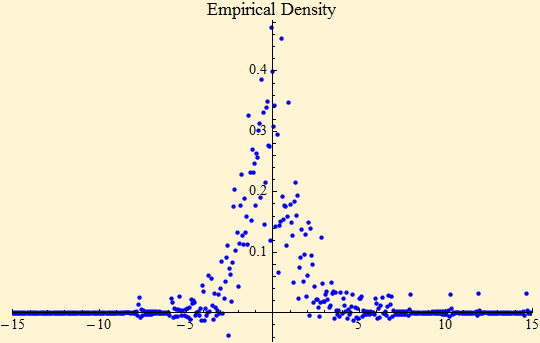
g1 = ListPlot[Transpose[{XTable[16, 8192], ReOrder[pdf]}], PlotRange -> {{-15, 15}, All}, PlotStyle -> Blue, PlotLabel -> "Empirical Density"]

The absolute amplitudes and the density show a lot of high frequency oscillation and beg to be smoothed.  It is easy to filter something in the transform domain.

sfilt = DFTCF[CharacteristicFunction[ NormalDistribution[0, 0.25 Sqrt[2]], #] &, 16, 8192];
scale = 8192/16;
pdf1 = Chop[InverseFourier[scale  sfilt ecf]];
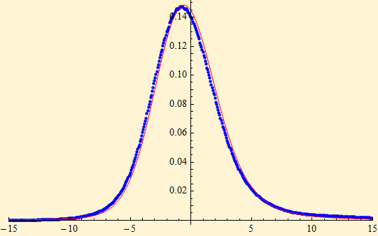
g2 = ListPlot[Transpose[{XTable[16, 8192], ReOrder[pdf1]}], PlotRange -> {{-15, 15}, All}, PlotStyle -> Blue];
g3 = Plot[SPDF[x, parm], {x, -15, 15}, PlotRange -> All, PlotStyle -> Red, PerformanceGoal -> "Speed"];
Show[g2, g3]

Choosing the right filter, however, is difficult.  Interestingly if the empirical characteristic function is multiplied by itself to create a distribution of summed random variables, it be comes smooth without filtering.  Here is the distribution of the sum of three random variables.  Since we are using a stable distribution we can calculate what the distribution of the sum of three random variables would be, shown in red.

pdf1 = Re[Chop[InverseFourier[(scale ecf)^3]]]/scale;
g2 = ListPlot[Transpose[{XTable[16, 8192], ReOrder[pdf1]}], PlotRange -> {{-15, 15}, All}, PlotStyle -> Blue];
g3 = Plot[SPDF[x, {1.7, 0.5, 3^(1/1.7), 0}], {x, -15, 15}, PerformanceGoal -> "Speed", PlotStyle -> Red];
Show[g2, g3]

© Copyright 2008 mathestate    Fri 7 Mar 2008