Convolution

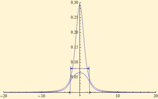
Convolution in the transform domain is simple multiplication.  Here is an example of convolution of symmetric stable distribution with a square wave, the amplitude is adjusted so that the area under the curve is 1, i.e. it is a statistical density function.

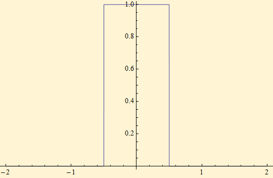
square[x_, w_] := (Sign[x + w/2] - Sign[x - w/2])/(2 w);
Plot[square[x, 1], {x, -2, 2}]

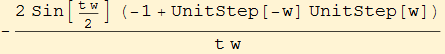
FourierTransform[square[x, w], x, t, Assumptions -> w ∈ Reals]
Limit[-1/(t w) Sqrt[2/Pi] Sin[t w/2] (-1 + UnitStep[-w] UnitStep[w]), t -> 0]

squaref[t_, w_] := -1/(t w) Sqrt[2/Pi] Sin[t w/2] (-1 + UnitStep[-w] UnitStep[w]);
squaref[0, w_] := -(-1 + UnitStep[-w] UnitStep[w])/Sqrt[2 Pi];
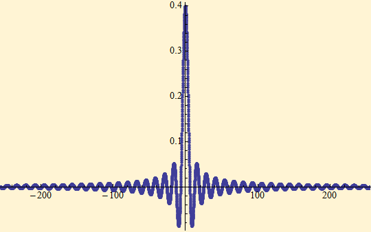
scale = 8192/16;
sqfilt =  scale  DFTCF[squaref[#1, 5] &, 16, 8192];
ListPlot[Transpose[{XTable[16, 8192], ReOrder[sqfilt]}], PlotRange -> {{-scale/2, scale/2}, All}]

scf = DFTCF[CF1c[#1, 1.3, 0, 1, 0] &, 16, 8192];
ListPlot[Transpose[{XTable[16, 8192], scale ReOrder[scf]}], PlotRange -> {{-scale/2, scale/2}, All}]

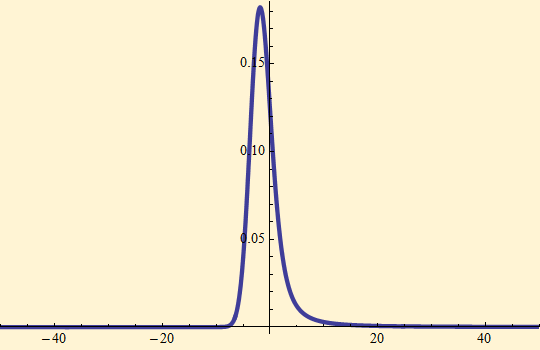
conv = Chop[InverseFourier[ scf sqfilt]];
g1 = ListPlot[Transpose[{XTable[16, 8192], ReOrder[conv]}], PlotRange -> {{-20, 20}, All}, Joined -> True, PlotStyle -> Blue];
conv = Chop[InverseFourier[ scf]];
g2 = ListPlot[Transpose[{XTable[16, 8192], ReOrder[conv]}], PlotRange -> {{-20, 20}, All}, Joined -> True];
conv = Chop[InverseFourier[sqfilt/scale]];
g3 = ListPlot[Transpose[{XTable[16, 8192], ReOrder[conv]}], PlotRange -> {{-20, 20}, All}, Joined -> True];
Show[g2, g3, g1]

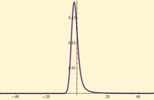
Convolution of two characteristic functions will give the characteristic function of the the sum of a random variable from each function.  The following will give the density of the sum of an S(1.3, 1, 1, 0;1) and a S(2 ,0, 1, 0;1) random variable.

scale = 8192/16;
skew = DFTCF[CF1c[#, 1.3, 1, 1, 0] &, 16, 8192];
nrml = scale DFTCF[CF1c[#, 2, 0, 1, 0] &, 16, 8192];
conv1 = InverseFourier[ skew nrml] // Chop;
g0 = ListPlot[Transpose[{XTable[16, 8192], ReOrder[conv1]}], PlotRange -> {{-50, 50}, All}, Joined -> True, PlotStyle -> Thickness[0.008]]

The convolution can be obtained very slowly with numerical integration.

AbsoluteTiming[g1 = Plot[NIntegrate[SPDF[t, {1.3, 1}, 1] SPDF[x - t, {2, 0}, 1], {t, -∞, ∞}, Method -> {Automatic, "SymbolicProcessing" -> 0}], {x, -50, 50}, PlotStyle -> Orange, PlotRange -> All];]
Show[g0, g1]

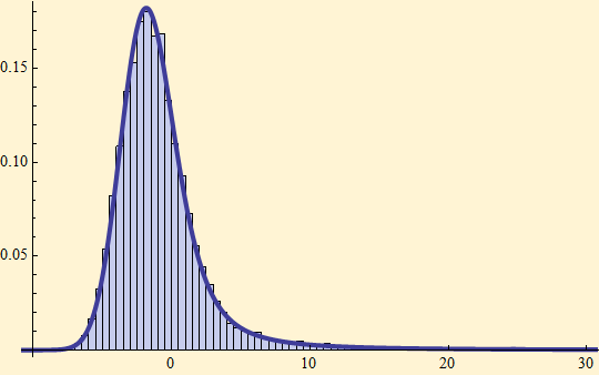
Obtain the result by simulation.

s = SRandom[10000, {1.3, 1}] + SRandom[10000, {2, 0}];
g2 = Histogram[s, HistogramScale -> 1, HistogramRange -> {-10, 30}];
Show[g2, g0, PlotRange -> {{-10, 30}, All}]

© Copyright 2008 mathestate    Fri 29 Feb 2008