Log Normal Stable Random Variables
We defined the lognormally scaled stable distribution as the distribution resulting from the product of a log normal random variable and a standardized stable random variable. The distribution has the properties that the tails are asymptotically the same as stable tails, but there is more mass in the center and mid arms of the distribution. The skewness factor is also significantly damped by the scaling. The δ parameter was added in a way that it remains the expectation of the distribution when α > 1.
The algorithm to construct a lognormal stable random variable is shown in Mathematica below. SRandom procedure generates a stable random variable and the location parameter is added after the multiplication.
LNStableRV[n_, {α_, β_, γ_, σ_, δ_}] := RandomReal[LogNormalDistribution[Log[γ], σ], n] SRandom[n, {α, β, 1, 0}] + δ;
The histograms show maximally skewed LNStable and Stable distributions with similar stable parameters, the shape of the distributions is quite different.

Below is the case of symmetric LNStable and Stable distributions. Note that the Stable distribution has more mass centrally and the tail behavior starts closer to the center of the distribution.

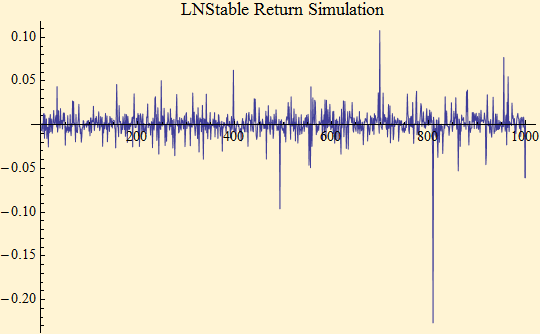
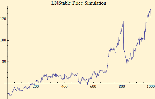
We can do price simulations in the same way we did for stable distributions. The parameter set is: {1.8, -0.08, 0.006, 0.5, Log[1.07]/250}.


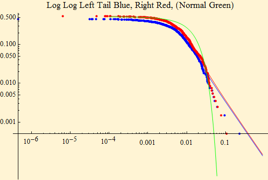
If we try to fit LNStable random variables with a stable distribution we find the same phenomenon we did with market data. As we have seen before we get a tail exponent, α, which is lower (heavier) than the data.

Stable fit parameters: {1.45258, 0.0350185, 0.0058299, 0.00104949}

© Copyright 2008 mathestate Mon 26 May 2008
