Fitting Market Data

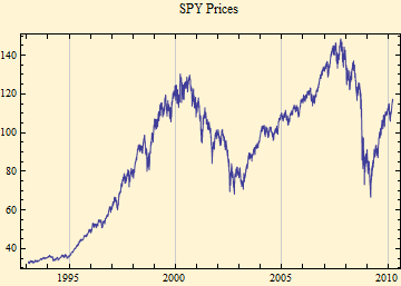
A reasonably accurate fit of stable parameters to a data set can be obtained by the maximum likelihood method.  Below are plots of the SPY prices since 1993, the calculated density function with histogram, and the empirical density and distribution.  The calculated fits are in blue.

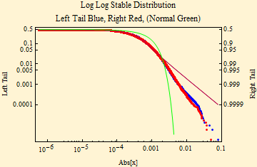
The fit of financial data to stable distributions has some problems.  Above we show some curves of the fit of SPY data to stable density and distribution curves.  Those pictures, however, don't well show the detail of the tails.  Below are the stable parameter fit using maximum likelihood method.  The plot beneath that shows a log-log fit to the cumulative distribution function; to align the tails, the absolute value of the left tail is shown in blue; the right tail is shown as 1- probability in red.  In this format stable distributions with α < 2, show linear parallel tails with the slope of minus α.  If β is zero the tails are superimposed (when β = ±1, the lighter tail is not linear).  The tail of a Normal distribution calculated from the sample is shown in green and is not linear.  The dots show the data points of the respective tails.

α	β	γ	δ
1.5633	-0.171349	0.00616486	0.000023598

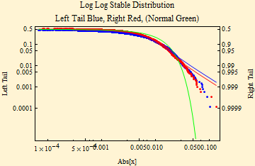
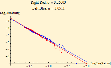
The actual data tails are too light with slope steeper than that of the fit.  When the actual slopes of the tails of the data are calculated from the data tails (upper and lower 2%), the tail exponents are far too high (graph below).  To fit stable laws tail exponents must be less than 2.  By the generalized central limit theorem sums of random variables from distributions with linear tail exponents that are less than two will converge to a stable distribution.  Those with higher tail exponents will converge to a Normal distribution on  summation.  Data with tail exponent higher than two cannot be from a stable distribution.

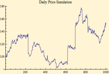
Conversely, if we take a simulation derived from the fit of financial data to a stable distribution with parameters such as above and reconstruct a price series, we find extreme changes more frequently than are ever found in a financial time series.  Thus the stable fit over estimates the frequency of extreme events, for financial data.  There is a dynamic demonstration of the graph below on the Wolfram Demonstrations Project.

Another problem in using a statistical distribution for financial data is that financial data are not completely random.  Below an autocorrelation plot of the SPY price series of log returns looks random, i.e. no observable autocorrelation.

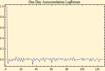
However, when you look at the same autocorrelation function with the absolute value of the log returns there is evidence of serial dependence in the data.

If you scramble the order of the same data above the serial dependent structure disappears.

The above phenomena could occur if the time series is not stationary, but has a varying scale factor.  The γ parameter of a stable distribution is proportional to the mean absolute deviation of the data.   To explore this in greater depth we will use higher resolution data, with prices collected every minute of the trading day.  The trading days are concatenated so there is no gap between a closing price and the next open.  The SPY series here starts in July 2007.

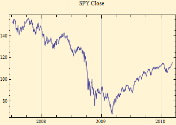
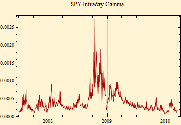
The plots above show the closing price for each day and the stable gamma calculated from the 391 minute by minute data points for each trading day.  Clearly there is a marked variation of the intraday scale factor, gamma.  Note also the opposite general slopes of the price and gamma tracings.  When we look at the autocorrelation function of the intraday data, a new level of structure is revealed.

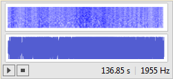
The upper (blue) series is the raw data.  There are two components, one is a cyclic change that occurs at the day to day level with a sharp spike at the return caused between the sequence of  a market close and a market open where actual physical time is not continuous.  Gradually the blue curve decays over time leaving a daily autocorrelation cycle that stays close to zero after the opening spike, with a fall after the open and a rise before the next close.  The red curve is the same data but each day's data has been divided by the intraday gamma, shown in the previous plot.   This removes the day to day serial dependent structure leaving only the intraday cycle.  Although it is not easy to see this extra structure when you look at a time series of returns, it is actually easy to hear it.  The display below converts the log return series to sound using the Mathematica function ListPlay.  When you listen to the data, you will notice the crescendo of amplitude seen in November, August, and January as well as the mechanical repetitive sound related to the intraday cycle.

Play Market Sound

Immediately below are the stable parameters of the minute by minute log returns and the log-log fit.  We se the same phenomenon of tails too light for the stable fit as we did in the day to day data, there are now 391 points for every day, yet the pattern is strikingly similar.

α	β	γ	δ
1.40774	3.19027*10^^-9	0.000332415	-3.2192*10^^-7

α	β	γ	δ
1.75942	-1.13624*10^^-7	1.01631	0.00360907

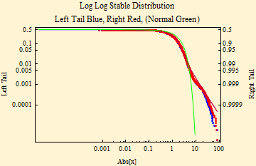
The plot and parameters immediately above shows the fit of the log returns that scaled by dividing by the daily gamma.  The division results in a gamma close to one as expected, but now the tail fit is much closer to the calculated stable fit.  The intraday cycle has been left and shows up as a obvious wiggle in the tail.  Note that the alpha parameter calculated with this data correction is now much higher.  

If we scale the intraday gamma to a daily gamma using the formula:

We find that gamma seems too high if we use the alpha from the uncorrected fit, but just about right if we use the alpha from the scaled data.

Scaled by α = 1.40774, γ-daily = 0.0230707

Scaled by α = 1.75942, γ-daily = 0.00988539

At the risk of torturing the data, we can use a similar strategy to remove the intraday cycle.  Here we fit the adjusted scale factor minute by minute through the day to a parabola for the correction.  For the sample we select only full trading days; for the fit we exclude the return from the previous close to the open.

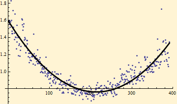
With this strategy we have removed all but the day to day spikes in the autocorrelation function and the oscillation in the tail fit.  The estimated parameters, {α, β} change only a little; {γ, δ} no longer have any meaning relative to our original data.

α	β	γ	δ
1.81142	1.30027*10^^-8	1.03815	0.00302009

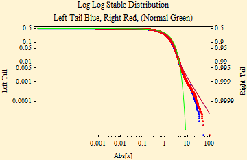
We have demonstrated some of the problems with fitting financial data to stable distributions.  Financial data are not from a stationary distribution.  There is some hope that the alpha parameter might be somewhat fixed with significantly higher value than obtained by the assumption that all the parameters are stationary, but this is not easy to prove.  A day to day variation of the scale factor confounds the problem.  It can be estimated and scaled away, but there is also a cyclic intraday pattern.  The daily variation also follows a quarterly earnings reporting cycle and is disturbed by other recurring events such as Federal Reserve Board meetings.  

Nevertheless it seems reasonable to postulate that the price formation process arises from sums of returns (or small price differences) that are driven by a fat-tailed distribution in market order books.  The apparent scale may vary by rapid changes in numbers of orders presented per unit time with a cascading effect that produces feedback in both numbers of new orders and the spacing of orders in the limit order books.  The process can quickly become complicated, but the data output by a market system suggests that sums of returns over intervals as short as a minute seem to converge to stable distributions which vary their parameters in a cyclic pattern during the trading day and with a serially dependent scale factor from day to day.  Such a system can be modelled and studied, but it does not have the convenience of simple mathematical laws that might be attributed to independent and identically distributed random variables.

Observation of the γ-parameter of the intra-day data, reveals that, although it shows a strong pattern of serial dependence, over longer time frames it might be modeled as a random variable with a lognormal distribution.  This leads to a mixture distribution, which we are studying, the LogNormalStable Distribution.   We have examined the model carefully with the most recent highly volatile data and it seems to be holding up extremely well.

Here is a link to calculate stable parameters for individual securities.

© Copyright 2010 mathestate    Wed 24 Mar 2010