Shifting and Scaling
Shifting the position of a density function is easy to accomplish in the probability domain, but there are times when one might want to accomplish the operations in the transform domain, while they are a little more complicated, they are ultimately multiplication operations.
For the examples a simple symmetric stable distribution will be used.
The DFTCF may also be used to map any function in the transform domain to a discrete FFT. Scale is the x-range in the probability domain; the range of x in the probability domain will be [-N/(2 SR), N/(2 SR)-1/SR].
sdft = DFTCF[CF1c[#1, 1.5, 0.5, 1, 0] &, 16, 8192];
conv = Chop[InverseFourier[sdft]];
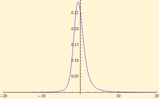
g1 = ListPlot[Transpose[{XTable[16, 8192], ReOrder[conv]}], PlotRange -> {{-20, 20}, All}, Joined -> True, PlotStyle -> Blue]

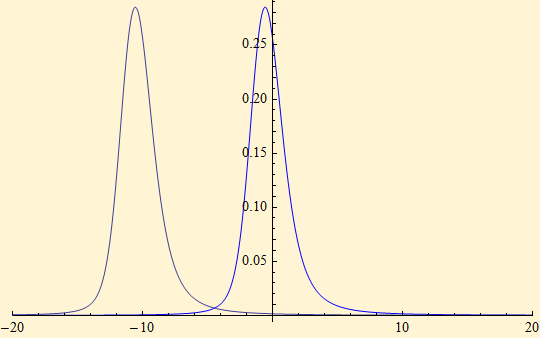
Changing the location in the transform domain, requires multiplication by the Fourier transform of the Dirac delta function.
TrigToExp[FourierTransform[ DiracDelta[x - d], x, t]]
![]()
It is a good idea to used compiled functions in DFTCF because they always output machine precision numbers and they are fast; the FFT works with machine numbers only. If a plain function is used, it should be wrapped with N or contain a machine precision number to ensure machine precision output, rather than a symbolic output.
shift = Compile[{t, d}, Exp[I t d]];
scale = 8192/16;
shift10 = scale DFTCF[shift[#1, -10] &, 16, 8192];(*the shift isn't scaled so it is multiplied by scale*)
conv1 = Chop[InverseFourier[ sdft shift10]];
g2 = ListPlot[Transpose[{XTable[16, 8192], ReOrder[conv1]}], PlotRange -> {{-20, 20}, All}, Joined -> True];
Show[g1, g2]

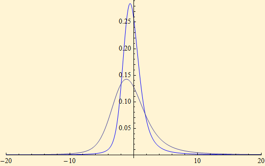
Scaling is a direct multiplication operation for the amplitude in the probability domain, but to keep the integral equal to one, the x-axis also has to be manipulated.
g2 = ListPlot[Transpose[{XTable[16, 8192] 2, ReOrder[conv]/2}], PlotRange -> {{-20, 20}, All}, Joined -> True];
Show[g1, g2]

Scaling as the discrete characteristic function is created is probably the best choice; in this case it could also be accomplished by setting the γ parameter to 2.
sdft = DFTCF[CF1c[2 #1, 1.5, 0.5, 1, 0] &, 16, 8192];
conv = Chop[InverseFourier[sdft]];
g2 = ListPlot[Transpose[{XTable[16, 8192], ReOrder[conv]}], PlotRange -> {{-20, 20}, All}, Joined -> True];
Show[g1, g2]


© Copyright 2008 mathestate Fri 29 Feb 2008
